Final Blog Post
Now that we have finally arrived at the end of coding period, I want to give you an overview of the whole project: what was the initial motivation and plan; what has been done; and what still would need to be implemented.
Code & documentation
Over the summer I worked on the IRAM.jl repository which aims at implementing ARPACK’s eigs function in pure Julia for nonsymmetric matrices. The documentation of the method can be found here.
Original plan
The aim was to implement a native Julia solver for the eigenvalue problem Ax = λx. In particular, the aim was to solve this problem for large and sparse, nonsymmetric matrices which would replace ARPACK’s eigs function. This helps reduce the dependency of Julia language on ARPACK. I will provide benchmarks comparing the performance of the native eigs versus ARPACK’s eigs. The aim at first was to get the method into the package IterativeSolvers.jl. However, it is also a possibility to just register the package separately.
Motivation
Benefits of implementing native replacement of eigs:
- Julia becomes a little more lightweight
- Native
eigscan be applied to different array types and different number types (BigFloats, DoubleFloats, etc.) - Native
eigsis more readable and easier to maintain than ARPACK’seigsthat is written in Fortran 90
Initial project outline
- IRAM for real and complex arithmetics with QR iterations through Givens rotations. DONE
- Finding multiple eigenpairs which requires locking of converged Ritz vectors. DONE
- Adding search targets for eigenvalues. DONE
- However, search targets are not implemented in the same way as in ARPACK. The method targets the eigenvalues that are largest in magnitude by default which has the highest convergence rate. If the user wants to target the eigenvalues that are the smallest in magnitude, they have to invert the problem as detailed in the documentation.
- Adding support for generalized eigenvalue problems.
- This functionality is not incorporated in the method either. Generalized eigenvalue problems can be solved if the user provides an input matrix that contains the effect of both matrices in the generalized eigenvalue problem. A detailed explanation can be found in the documentation.
In addition:
- Making the implementation fully native. PARTLY DONE
- Native Julia implementations for the
schurfact!call and theeigvalscall have been implemented. However,schur_to_eigenis not yet fully native.
- Native Julia implementations for the
Major developments
During the time period, the project was jointly developed with my mentor and a lot of communication took place on Slack. I will list here the key PRs that I was a part of:
- Computing the QR decomposition through Givens rotations and using this in
implicit_restart!: #2, #4 - Locking of Ritz vectors: #7
- QR step made implicit: #10
- Added native Julia implementations of computing Schur factorization for a Hessenberg matrix and computing eigenvalues from the Schur form: #28, #30
- Transform Schur form into eigenvectors: #49
What’s left to do?
Method-wise:
- The criterion for convergence should be changed to how it is implemented in
eigs.eigsconsiders a Ritz valueθconverged when its residual||Av - vθ||is smaller than the product oftolandmax(ɛ^{2/3}, |θ|), whereɛ = eps(real(eltype(A)))/2is LAPACK’s machine epsilon. Nativepartial_schurconsiders the Ritz value converged only when the subdiagonal of the Hessenberg matrix in smaller than the user provided tolerancetol.
Functionality-wise:
partial_schurreturns the partial Schur decomposition. What still needs to be done is to implement a native Julia implementation for computing the eigenvectors and eigenvalues from the partial Schur decomposition. Computing eigenvalues is quite straightforward and is currently implemented ineigvalues. However, computing the eigenvectors requires taking into account some stability considerations that are not currently implemented. Hence, currently the implementation only returns the partial Schur decomposition, andschur_to_eigenthen computes the eigenvalues and eigenvectors by usingeigen.
Performance-wise & stability-wise:
- The code needs to be profiled in order to find areas of improvement. The method should closely follow the implementation of
eigs, however sometimes nativepartial_schurseems to be much slower thaneigs. In fact, in some cases the nativepartial_schurrequires more iterations thaneigsto find the eigenvalues of the same matrix which suggests that there are differences between the methods themselves. A likely explanation for this is differences in the stopping criterion. - Currently known performance considerations
- Temporary variables could be refactored in order to reduce the amount of allocations
- In
backward_subst!, the case when the method computes eigenvectors for conjugate eigenvalues could be implemented in such a way that we stay in real arithmetic throughout the whole computation
- Stability considerations for
backward_subst!(e.g. smallest value for which it is safe to divide). The aim is to have a similar implementation as in LAPACK.
How to use it?
Example 1
julia> using IRAM, LinearAlgebra
# Generate a sparse matrix
julia> A = spdiagm(-1 => fill(-1.0, 99), 0 => fill(2.0, 100), 1 => fill(-1.001, 99));
# Compute Schur form of A
julia> schur_form,  = partial_schur(A, min = 12, max = 30, nev = 10, tol = 1e-10, maxiter = 20, which=LM());
julia> Q,R = schur_form.Q, schur_form.R;
julia> norm(A*Q - Q*R)
6.336794280593682e-11
# Compute eigenvalues and eigenvectors of A
julia> vals, vecs = schur_to_eigen(schur_form);
# Show that Ax = λx
julia> norm(A*vecs - vecs*Diagonal(vals))
6.335460143979987e-11
In the partial_schur function call, A is the n×n matrix whose eigenvalues and eigenvectors you want; min specifies the minimum dimension to which the Hessenberg matrix is reduced after implicit_restart!; max specifies the maximum dimension of the Hessenberg matrix at which point iterate_arnoldi! stops increasing the dimension of the Krylov subspace; nev specifies the minimum amount of eigenvalues the method gives you; tol specifies the criterion that determines when the eigenpairs are considered converged (in practice, smaller tol forces the eigenpairs to converge even more); maxiter specifies the maximum amount of restarts the method can perform before ending the iteration; and which is a Target structure and specifies which eigenvalues are desired (Largest magnitude, smallest real part, etc.).
The function call partial_schur returns a partial Schur decomposition AQ = QR of the matrix A where the upper triangular matrix R is of size nev×nev and the unitary matrix Q is of size n×nev. schur_to_eigen then computes the eigenvalues and eigenvectors of matrix A from the Schur decomposition.
Example 2: Formation of sound waves in mouth
The same method can be applied to solving the eigenfunctions of the Helmholtz equation c²Δu + k²u = 0 where c is a constant and k is the wavenumber, which is a time-independent description of the behaviour of waves. The problem can be discretized into small areas in the domain that are piece-wise constant. Then the problem takes the form Ax = λBx, which is a generalized eigenvalue problem.
The discretization was done so that the matrices A and B became of size 1176×1176. This probelm can now be solved with eigs where the eigenvalues of smallest magnitude are targeted. Moreover, with our boundary conditions the problem is a square eigenvalue problem which leads to nonsymmetric A for which the native implementation is optimized.
Let the domain be mouth shaped as shown in Figure 1. We have an open boundary condition on the left side c*du/dn + iku = 0 which lets the waves pass through the boundary. On the rest of the sides, we have a fixed boundary condition u = 0. Below, two eigenfunctions are visualized. This is an elementary model of how sound waves can form in the mouth.
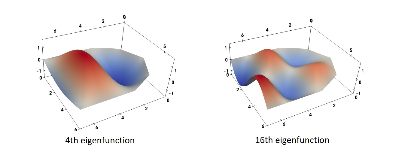 Figure 1. Two eigenfunctions of the Helmholtz equation in a mouth shaped domain.
Benchmarks
The native partial_schur was benchmarked against ARPACK’s eigs. However, it is difficult to compare benchmarks due to differences in the stopping criterion. In any case, it seems that even with a quite relaxed stopping criterion (1e-5) for natve partial_schur, it still has poorer performance compared to native eigs. However, an absolute criterion of 1e-5 might still be very strict when eigenvalues are very large. In an attempt to ignore the effect of these different stopping criterions, the time taken per one matrix-vector product is computed.
In these benchmarks, the two methods solve a generalized eigenvalue problem with sparse tridiagonal 1948×1948 matrix targeting eigenvalues that are smallest in magnitude.
ARPACK’s eigs:
BenchmarkTools.Trial:
  memory estimate:  23.03 MiB
  allocs estimate:  2214
  --------------
  minimum time:     83.047 ms (2.16% GC)
  median time:      98.686 ms (2.12% GC)
  mean time:        105.291 ms (4.37% GC)
  maximum time:     201.714 ms (45.27% GC)
  --------------
  samples:          48
  evals/sample:     1
  --------------
  Amount of matrix-vector products: 66
  Mean time per matrix-vector product: 1.5953 ms
Native partial_schur (tol = 1e-10):
BenchmarkTools.Trial:
  memory estimate:  62.23 MiB
  allocs estimate:  5990
  --------------
  minimum time:     451.928 ms (0.45% GC)
  median time:      567.831 ms (0.47% GC)
  mean time:        575.171 ms (2.29% GC)
  maximum time:     748.566 ms (0.44% GC)
  --------------
  samples:          9
  evals/sample:     1
  --------------
  Amount of matrix-vector products: 473
  Mean time per matrix-vector product: 1.2160 ms
Native partial_schur (tol = 1e-5):
BenchmarkTools.Trial:
  memory estimate:  29.88 MiB
  allocs estimate:  2836
  --------------
  minimum time:     222.053 ms (0.34% GC)
  median time:      302.852 ms (0.48% GC)
  mean time:        328.230 ms (2.07% GC)
  maximum time:     600.037 ms (0.41% GC)
  --------------
  samples:          16
  evals/sample:     1
  --------------
  Amount of matrix-vector products: 231
  Mean time per matrix-vector product: 1.4209 ms
Native partial_schur (tol = 1e-1):
BenchmarkTools.Trial:
  memory estimate:  4.34 MiB
  allocs estimate:  336
  --------------
  minimum time:     20.436 ms (0.00% GC)
  median time:      24.677 ms (0.00% GC)
  mean time:        29.240 ms (2.58% GC)
  maximum time:     112.312 ms (0.00% GC)
  --------------
  samples:          173
  evals/sample:     1
  --------------
  Amount of matrix-vector products: 22
  Mean time per matrix-vector product: 1.3291 ms
In conclusion, the time taken per each matrix-vector product is approximately the same between ARPACK’s eigs and the native Julia partial_schur. This suggests that the difference in the running time is caused by differences in the mathematical methods, and that the stopping criterion plays a role here.